vizWithSCE
Kwame Forbes
05/14/2021
vizWithSCE.RmdIntroduction
vizWithSCE is an R package that assists with the visualization of the integration of bulk DE results tables with pre-processed scRNA-seq datasets available on Bioconductor. vizWithSCE currently takes two arguments, a list containing res, dds, and a SingleCellExperiment (sce) as selected by the user and a second argument which. The which argument is the gene to use for the violin plot, represented as a number that corresponds to the gene with the n-th smallest p-value, e.g., 1 for the gene with lowest p-value, etc.
Run DESeq2 to obtain bulk DE results
We first load gene-summarized RNA-seq counts.
library(airway)For our workflow, we used the bulk dataset “airway”, which contains four human airway smooth muscle cell lines treated with dexamethasone, a steroid used to treat inflammation. This pre-processed dataset is available on Bioconductor. Here we filter to at least 3 samples with a count of 10 or higher, and then perform differential expression analysis.
Here, we changed the rownames to match the format of the sce.
library(DESeq2)
data(gse)
levels(gse$condition) <- c("untrt", "trt")
dds <- DESeqDataSet(gse, design = ~donor + condition)
keep <- rowSums(counts(dds) >= 10) >= 3
dds <- dds[keep,]
dds <- DESeq(dds)
res <- results(dds)
rownames(res) <- sub("\\..*","",rownames(res))
## using 'avgTxLength' from assays(dds), correcting for library size
Run integrateWithSingleCell
We run integrateWithSingleCell and pick number 8 from the dataset selection as our single-cell dataset. Within PBMC there are nine different scRNA-seq datasets. We chose the dataset pbmc4k, which contains roughly 4 thousand cells. This pre-processed dataset is available on Bioconductor.
dat <- integrateWithSingleCell(res, dds)Label cell types or clusters
We use scater’s logNormCounts function to add normalized data to the sce. We create a copy of the sce object in order to perform cell type labeling.
library(scater)
dat$sce <- scater::logNormCounts(dat$sce)
sce2 <- dat$sce
We convert the rownames from Ensembl to gene symbols, to match with the cell annotation reference dataset, described below.
We use celldex which is a database of reference expression datasets along with SingleR to provide cell type recognition. Now dat contains labels of different cell types.
Use vizWithSCE for visualization
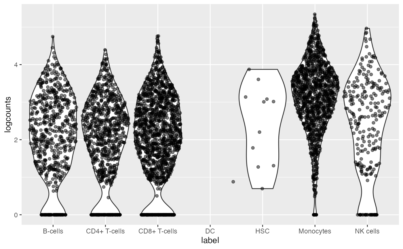
We use vizWithSCE to pick the second gene by smallest p-value, and make a violin plot over the cell labels from SingleR. DUSP1 is known to play a role in response to environmental stress, and is most highly expressed in monocytes according to the single cell data.
library(vizWithSCE)
vizWithSCE(dat, which=2)
Future direction
- We are currently planning to add more features, including other types of plots, allowing users to further explore the intersection of the two datasets. We seek to add multiple gene plots, e.g. dotplots or heatmaps of sets of DE genes.
- We are considering statistical tests of the distribution of expression across cell types for sets of DE genes, e.g. up-regulated vs down-regulated DE genes.
- We will explore launching iSEE from our worklow, a well-developed package for interactive exploration of SCE datasets.
Session info
## R version 4.0.4 (2021-02-15)
## Platform: x86_64-apple-darwin17.0 (64-bit)
## Running under: macOS Big Sur 10.16
##
## Matrix products: default
## BLAS:   /Library/Frameworks/R.framework/Versions/4.0/Resources/lib/libRblas.dylib
## LAPACK: /Library/Frameworks/R.framework/Versions/4.0/Resources/lib/libRlapack.dylib
##
## locale:
## [1] en_US.UTF-8/en_US.UTF-8/en_US.UTF-8/C/en_US.UTF-8/en_US.UTF-8
##
## attached base packages:
## [1] parallel  stats4    stats     graphics  grDevices utils     datasets
## [8] methods   base
##
## other attached packages:
##  [1] scater_1.18.6               ggplot2_3.3.3
##  [3] TENxPBMCData_1.8.0          HDF5Array_1.18.1
##  [5] rhdf5_2.34.0                DelayedArray_0.16.2
##  [7] Matrix_1.3-2                SingleCellExperiment_1.12.0
##  [9] SummarizedExperiment_1.20.0 Biobase_2.50.0
## [11] GenomicRanges_1.42.0        GenomeInfoDb_1.26.2
## [13] IRanges_2.24.1              S4Vectors_0.28.1
## [15] BiocGenerics_0.36.0         MatrixGenerics_1.2.1
## [17] matrixStats_0.58.0          vizWithSCE_0.0.5
##
## loaded via a namespace (and not attached):
##   [1] ggbeeswarm_0.6.0              colorspace_2.0-0
##   [3] ellipsis_0.3.1                rprojroot_2.0.2
##   [5] scuttle_1.0.4                 XVector_0.30.0
##   [7] BiocNeighbors_1.8.2           fs_1.5.0
##   [9] farver_2.1.0                  bit64_4.0.5
##  [11] interactiveDisplayBase_1.28.0 AnnotationDbi_1.52.0
##  [13] fansi_0.4.2                   splines_4.0.4
##  [15] sparseMatrixStats_1.2.1       cachem_1.0.4
##  [17] geneplotter_1.68.0            knitr_1.31
##  [19] polyclip_1.10-0               jsonlite_1.7.2
##  [21] annotate_1.68.0               dbplyr_2.1.1
##  [23] ggforce_0.3.3                 shiny_1.6.0
##  [25] BiocManager_1.30.10           compiler_4.0.4
##  [27] httr_1.4.2                    assertthat_0.2.1
##  [29] fastmap_1.1.0                 BiocSingular_1.6.0
##  [31] later_1.1.0.1                 tweenr_1.0.2
##  [33] htmltools_0.5.1.1             tools_4.0.4
##  [35] rsvd_1.0.3                    gtable_0.3.0
##  [37] glue_1.4.2                    GenomeInfoDbData_1.2.4
##  [39] dplyr_1.0.5                   rappdirs_0.3.3
##  [41] Rcpp_1.0.6                    jquerylib_0.1.3
##  [43] pkgdown_1.6.1                 vctrs_0.3.6
##  [45] rhdf5filters_1.2.0            ExperimentHub_1.16.0
##  [47] DelayedMatrixStats_1.12.3     xfun_0.22
##  [49] stringr_1.4.0                 beachmat_2.6.4
##  [51] irlba_2.3.3                   mime_0.10
##  [53] lifecycle_1.0.0               XML_3.99-0.5
##  [55] AnnotationHub_2.22.0          zlibbioc_1.36.0
##  [57] MASS_7.3-53                   scales_1.1.1
##  [59] ragg_1.1.2                    promises_1.2.0.1
##  [61] RColorBrewer_1.1-2            yaml_2.2.1
##  [63] curl_4.3                      gridExtra_2.3
##  [65] memoise_2.0.0                 sass_0.3.1
##  [67] stringi_1.5.3                 RSQLite_2.2.3
##  [69] highr_0.8                     BiocVersion_3.12.0
##  [71] genefilter_1.72.1             desc_1.3.0
##  [73] BiocParallel_1.24.1           rlang_0.4.10
##  [75] pkgconfig_2.0.3               systemfonts_1.0.1
##  [77] bitops_1.0-6                  evaluate_0.14
##  [79] lattice_0.20-41               purrr_0.3.4
##  [81] Rhdf5lib_1.12.1               labeling_0.4.2
##  [83] bit_4.0.4                     tidyselect_1.1.0
##  [85] magrittr_2.0.1                DESeq2_1.30.1
##  [87] R6_2.5.0                      generics_0.1.0
##  [89] DBI_1.1.1                     pillar_1.6.0
##  [91] withr_2.4.1                   survival_3.2-7
##  [93] RCurl_1.98-1.2                tibble_3.1.0
##  [95] crayon_1.4.1                  utf8_1.1.4
##  [97] BiocFileCache_1.14.0          rmarkdown_2.7
##  [99] viridis_0.5.1                 locfit_1.5-9.4
## [101] grid_4.0.4                    blob_1.2.1
## [103] digest_0.6.27                 xtable_1.8-4
## [105] httpuv_1.5.5                  textshaping_0.3.3
## [107] munsell_0.5.0                 viridisLite_0.3.0
## [109] beeswarm_0.3.1                vipor_0.4.5
## [111] bslib_0.2.4